Simple anomaly detection using MAD
2024-04-21 — 5 min read
It can be very useful (and at times critical) to be able to spot unusual values or rapid behaviour changes in a system, especially where the data is expected to remain stable with no underlying long-term trends. In mobile gaming, for example, a sudden change in the number of active players might mean there is a bug causing the app to crash, so we need to detect this fast!
Median Absolute Deviation (MAD) anomaly detection is a robust technique used to identify outliers or anomalous changes in a dataset. Its main advantages lie in the fact that it is non-parametric, is simple to calculate, and less sensitive to extreme values compared to methods that rely on the mean and standard deviation. Instead, MAD anomaly detection is based on the median and median absolute deviation which are more resistant to outliers.
Calculations and worked example
Imagine that we run an automatic sensor monitoring the flow of traffic along a road, and counting the number of cars that pass each minute. During normal operation we might expect the number of cars per minute to remain roughly constant.
However, if there is a sudden increase in traffic this could lead to congestion problems, and so we should create an alert to direct drivers on other routes. Conversely, a sudden drop in traffic could indicate an accident or blockage further up the road. Any sudden change in the number of cars indicates that something is amiss - we want to be alerted to any significant deviation from the norm!
Suppose we have recorded the following number of cars per minute over the last 10 minutes: $$ 5,6,4,8,6,5,8,5,6,11 $$ Is the most recent value, 11 cars per minute, an anomaly?
First, we calculate the median value by ordering the values finding the middle value. Because we have an even number of values, we take the average of the middle two: $$ 4,5,5,5,\mathbf{6},\mathbf{6},6,8,8,11 $$ The median is 6.
Next we find the absolute deviation of each point from the median: $$ 2,1,1,1,0,0,0,2,2,5 $$ ...and again find the median value: $$ 0,0,0,1,\mathbf{1},\mathbf{1},2,2,2,5. $$ Therefore the median absolute deviation (MAD) for this sample is 1.
If the underlying data is normally distributed then multiplying the MAD by 1.4826 will approximate the standard deviation, \(\sigma\): we can define an adjusted MAD as $$ \text{MAD}_\text{adjusted} = 1.4826 \cdot \text{MAD}. $$
We can label a value as an outlier if it exceeds the MAD by some threshold, \(k\cdot\text{MAD}\). The choice of \(k\) may depend on what you want to class as an anomaly, and you may choose different thresholds depending on the shape of the underlying data.
In this example, let's assume that the data is normally distributed, so taking a threshold of \(k\cdot\text{MAD}_\text{adjusted}\) will represent a point that lies three standard deviations from the mean: $$\begin{eqnarray} \text{threshold} &= 3\cdot\text{MAD}_\text{adjusted} \\ &= 3\times 1.4826 \cdot \text{MAD} \\ &= 4.4478\cdot \text{MAD}. \end{eqnarray} $$
In our example \(\text{MAD} = 1\): the most recent measurement of 11 cars per minute had an absolute deviation of 5, which is bigger than our threshold, and so we have detected an anomaly!
MAD anomaly detection in action
We can apply MAD anomaly detection to a continuous stream of data, by calculating MAD for a rolling window and checking if the most recent value exceeds the threshold. The figure below shows this in action!
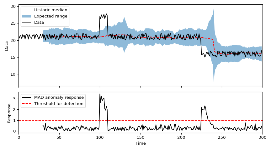
In the top panel, simulated data is shown by the black line. For the most part this random noise about a stable mean; however there are two features that could be considered anomalous based on the previous values: first, there is a short impulsive increase in the value for a few samples before it returns to normal; later, the average value of the data suddenly and permanently decreases. The red dashed line shows the median value of the last 30 samples.
As in the cars example, I have used a threshold of \(4.4478\cdot \text{MAD}\) and used this to show the expected range at any given time by the blue shaded area.
In the lower panel, the black line shows the "response" of this anomaly detection system which is a measure of how far the current value deviates from the rolling median. The response is calculated according to $$ \text{Response} = \frac{|\text{current value} - \text{rolling median}|}{ 4.4478\cdot \text{MAD} } $$
The horizontal red dashed line in the lower panel shows the threshold. At both times where there is a disturbance, there is a strong positive response that crosses the threshold, followed by a rapid decay. All data for which the response is above the threshold will be flagged as anomalous - in the real world, we could use this to trigger an alert that something unexpected has happened.
Summary
To summarise the steps we take to use MAD for outlier detection:
- Calculate the median value. If using in a time series data application, use a window of the most recent values;
- Calculate the absolute deviation of each point from the median
- Calculate the median absolute deviation (MAD): Calculate the median of the absolute deviations calculated in step 2. This gives you a measure of the typical distance between each data point and the median.
- Define a threshold: multiply the MAD by a threshold value is to determine which data points are considered anomalies. Typical values lie between 3 and 5 times, but the choice depends on the desired sensitivity and underlying data distribution.
- Identify anomalies: Compare each data point's deviation from the median to the threshold. If the deviation exceeds the threshold, the data point is flagged as an anomaly.
Detecting outliers and anomalous data is often critical requirement, and using MAD provides a simple yet robust solution. While it may require some fine tuning, it can be combined with other anomaly detection methods to acheive solid results across different systems. One of its key advantages is how easily explainable it is. It can be very quickly implemented to provide key insights into your data!
Further reading
- Median Absolute Deviation (Wikipedia)
- Anomaly Detection with Median Absolute Deviation (Influx Data)
- Identifying Outliers using MAD (Real Statistics)