Geometry of the Rotating Vector Model
2024-07-25 — 10 min read
Note: because this page contains long equations, it is best viewed on desktop.
The Rotating Vector Model
This page is dedicated to the derivation of one of the models of the geometry of radio pulsars I relied upon during my PhD - I have been meaning to formally write down the derivation for some time, and have finally got round to doing so. First, a little background!
The radio emission from pulsars typically shows a large amount of linear polarisation, especially in younger stars. The angle of this polarisation, the "position angle" (PA) is seen to change as the star rotates. Because pulsars have extremely strong magnetic fields, the change in the PA is thought to be associated with the changing orientation of the magnetic field lines with respect to the observer's line of sight.
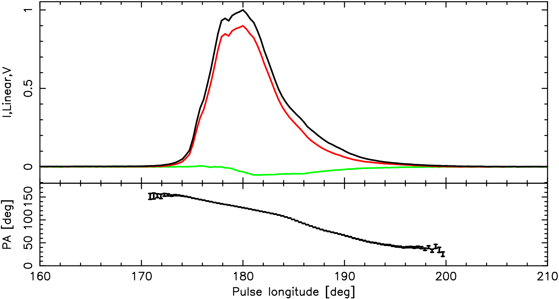
When plotted as a function of the star's rotation, or "pulse longitude", the position angle traces out a characteristic S-shaped curve. An example can be seen in the figure below, which shows the pulse profile and smooth PA curve of the Vela pulsar in the lower panel.
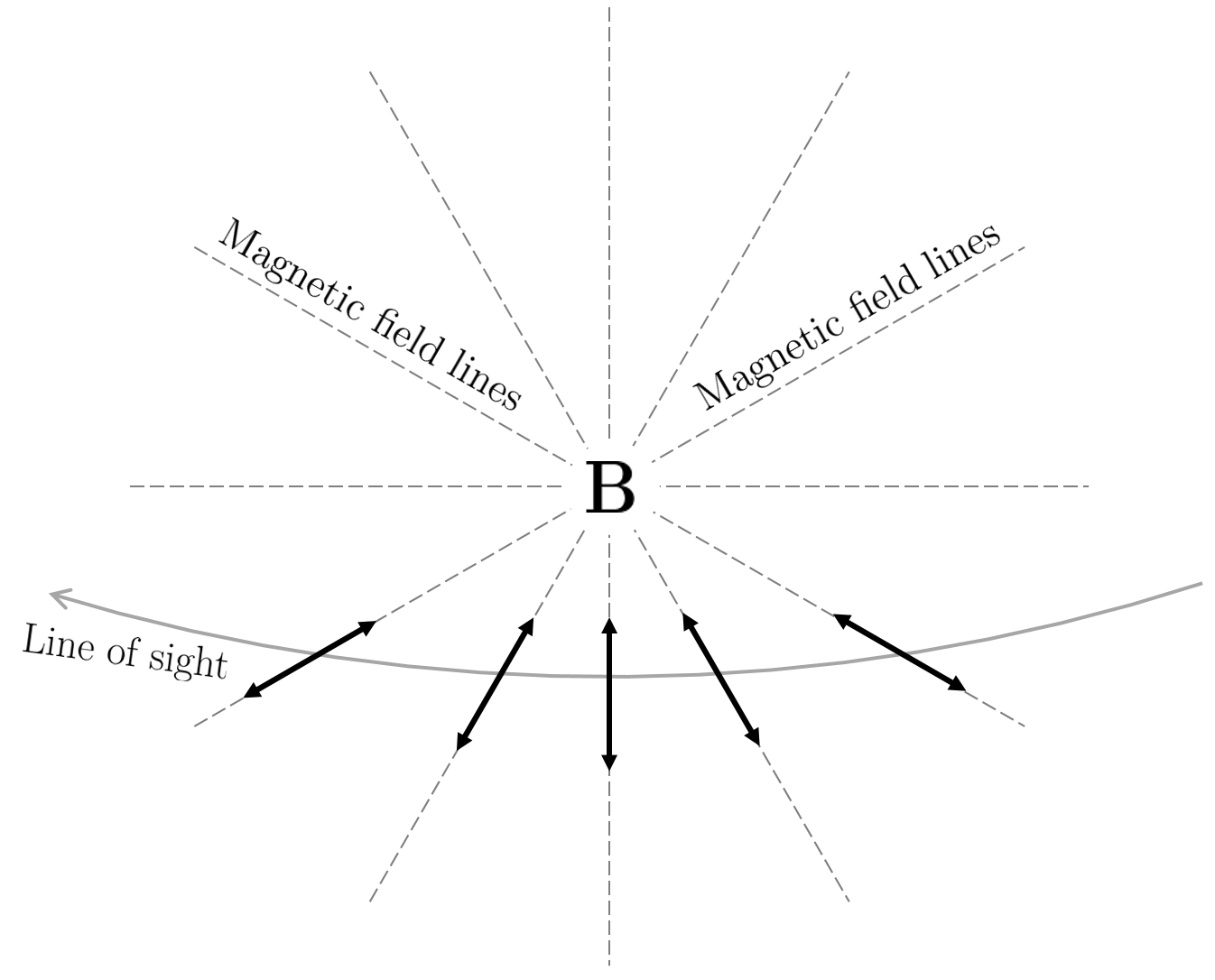
Radhakrishnan & Cooke (1969) showed that the PA curve can be fit by a simple geometric model they termed the Rotating Vector Model (RVM), built upon the following assumptions:'
- Each magnetic field line lies in a single plane containing the magnetic axis (for example a static dipolar field)
- This plane defines the linear polarisation direction of any radiation emitted in its vicinity.
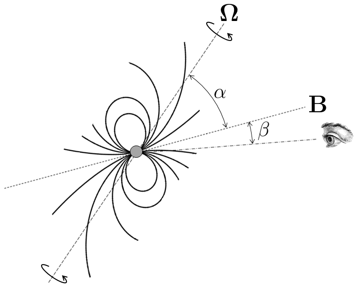
Komesaroff (1970) showed that the change in position angle, \(\psi\), as a function of the pulse longitude, \(\phi\), can be described by $$ \tan(\psi-\psi_0) = \frac{\sin(\phi-\phi_0)\sin\alpha}{\sin(\alpha + \beta)\cos\alpha - \cos(\alpha+\beta)\sin\alpha\cos(\phi-\phi_0)} $$ which is a smooth S-shaped curve with an inflection point at \((\phi_0,\ \psi_0) \). The angle \(\alpha\) is the inclination angle between the stars magnetic and rotation axes, and \(\beta\) is the impact angle between the magnetic axis and the observer's line of sight as the pulsar rotates.
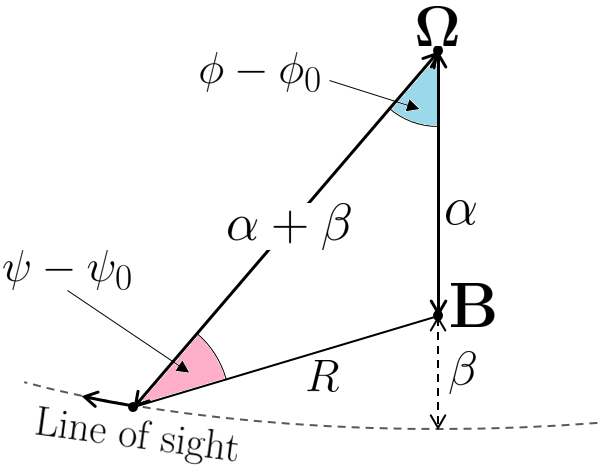
Overall, we can draw the full geometry of the Rotating Vector Model by defining a triangle on the surface of a sphere between three points: the pulsar's rotation axis, the magnetic axis, and the footprint of the observer's line of sight.
Spherical geometry rules
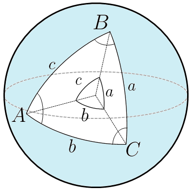
In order to derive the RVM equation given by Komesaroff, we must make use of two trigonometric identies for spherical geometry. These are the spherical sine rule: $$ \frac{\sin A}{\sin a} = \frac{\sin B}{\sin b} = \frac{\sin C}{\sin c} $$ ...and the spherical cosine rule: $$ \cos a = \cos b \cos c + \sin b \sin c \cos A. $$ These apply to a triangle drawn on the surface of a sphere as below, where each side is a great circle arc (the shortest path between two points on the surface of a sphere: a segment of a great circle, which is a circle on the sphere's surface whose center coincides with the center of the sphere).
Deriving the RVM
There are three equations we start with, which are simply the spherical sine and cosine rules applied to the triangle that defines the pular geometry:
\begin{equation}
\frac{\sin(\psi-\psi_0)}{\sin\alpha} = \frac{\sin(\phi-\phi_0)}{\sin R}
\end{equation}
\begin{equation}
\cos\alpha = \cos R \cos(\alpha+\beta)+\sin R \sin(\alpha+\beta)\cos(\psi - \psi_0)
\end{equation}
\begin{equation}\label{test}
\cos R = \cos(\alpha+\beta)\cos\alpha+\sin(\alpha+\beta)\sin\alpha\cos(\phi - \phi_0)
\end{equation}
First, we rearrange equations (1) and (2) to bring only the \(\psi\) terms to the left-hand side:
\begin{equation}
\sin(\psi-\psi_0)= \frac{\sin(\phi-\phi_0)\sin\alpha}{\sin R}
\end{equation}
\begin{equation}
\cos(\psi-\psi_0) = \frac{\cos\alpha - \cos R \cos(\alpha+\beta)}{\sin R \sin(\alpha+\beta)}
\end{equation}
Next, we divide (4) by (5) and cancel out the \(\sin R\) terms:
\begin{align}
\tan(\psi-\psi_0) &= \frac{\sin(\phi-\phi_0)\sin\alpha\sin(\alpha+\beta)\enclose{updiagonalstrike}{\sin R}}{\enclose{updiagonalstrike}{\sin R}\cos\alpha - \enclose{updiagonalstrike}{\sin R} \cos R \cos(\alpha + \beta)} \\[16pt]
&= \frac{\sin(\phi-\phi_0)\sin\alpha\sin(\alpha+\beta)}{\cos\alpha - \cos R \cos(\alpha + \beta)}
\end{align}
Substituting in Eq. (3) for \( \cos R \). Then, we can cancel the \(\sin(\alpha+\beta)\) terms to end up with the final RVM equation:
\begin{align}
\tan(\psi-\psi_0) &= \frac{\sin(\phi-\phi_0)\sin\alpha\sin(\alpha+\beta)}{\cos\alpha - \cos^2(\alpha + \beta)\cos\alpha - \sin(\alpha+\beta)\cos(\alpha+\beta)\sin\alpha\cos(\phi-\phi_0)} \\[16pt]
& = \frac{\sin(\phi-\phi_0)\sin\alpha\sin(\alpha+\beta)}{(1 - \cos^2(\alpha + \beta))\cos\alpha - \sin(\alpha+\beta)\cos(\alpha+\beta)\sin\alpha\cos(\phi-\phi_0)} \\[16pt]
& = \frac{\sin(\phi-\phi_0)\sin\alpha\enclose{updiagonalstrike}{\sin(\alpha+\beta)}}{\sin^\enclose{updiagonalstrike}{2}(\alpha + \beta)\cos\alpha - \enclose{updiagonalstrike}{\sin(\alpha+\beta)}\cos(\alpha+\beta)\sin\alpha\cos(\phi-\phi_0)} \\[16pt]
\tan(\psi-\psi_0) &= \frac{\sin(\phi-\phi_0)\sin\alpha}{\sin(\alpha + \beta)\cos\alpha - \cos(\alpha+\beta)\sin\alpha\cos(\phi-\phi_0)}.
\end{align}
We have derived the equation behind the Rotating Vector Model using simple spherical geometry and trigonometric identies. I hope this was interesting, and that it proves a useful for future students and for the simply curious!
Further reading
- Radhakrishnan V., Cooke D. J., 1969, Astrophysics Letters, 3, 225
- Komesaroff M. M., 1970, Nature, 225, 612
- Pulsar Astronomy (Lyne and Graham-Smith, 4th ed.)
- Chapter 1.2 of my PhD thesis!