Simulated annealing for global optimisation

2024-10-31 — 8 min read

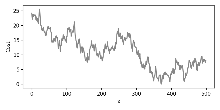
Simulated annealing is a surprisingly simple yet very robust technique used to find the global optimum of a complicated objective function. It is inspired by the process of annealing in metallurgy, where a hot material is allowed to cool over a long period of time as a way of reducing its internal defects.

The algorithm is a stochastic process that explores potential solutions to an objective function, moving between states probabilistically depending on the relative improvement of a trial solution over the current solution. The fact it can sometimes move to a worse state allows it to escape local minima that could otherwise trap other gradient-based methods.

An example of a noisy function with lots of local minima. Normal gradient-based optimisation methods would fail to find the lowest point on the curve, but simulated annealing might succeed.

It works by slowly reducing the "temperature" of a system during which it tests out different neighbouring solutions to its current state. If a trial solution is better than the current one then the system jumps straight to that new state. If the trial solution is worse, then it can still jump to that state but only with some probability, $P < 1$. The temperature influences this transition probability: higher temperatures mean the system is more likely to explore worse solutions.

Over time the temperature is reduced according to a "cooling schedule", making the system less likely to accept poor solutions. This means that eventually the system will settle down into the "best" (lowest cost) state.

Components of simulated annealing

The simulated annealing algorithm has several crucial components that work together to perform the optimisation. Each part mimics aspects of the physical annealing process in materials, where heat and gradual cooling allow particles to settle into a low-energy state. Here are the main features:

Objective Function

The objective function is the thing to be optimised. When simulated annealing is appropriate the objective function is usually a high-dimensional (has a lot of parameters), complicated (non-linear) function and can be quantified by a single measure. It may be discrete or combinatorial, for example the travelling salesman problem or the layout of a factory to maximise efficiency.

Neighbourhood structure

There must be the ability for the system to explore neighbouring states of the objective function by making small adjustments to the parameters subject to any constraints upon them.

Cooling schedule

The cooling schedule dictates how the temperature of the system is adjusted over time. The temperature starts high and decreases over successive iterations, slowly to avoid the system converging too quickly (to a suboptimal solution), but not too slow that the algorithm becomes inefficient. Commonly chosen cooling schedules include linear, exponential, or logarithmic decays, and adaptive cooling is sometimes used to adjust the schedule according to the behaviour of the objective function.

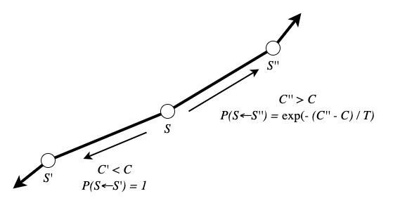
Acceptance probability

A key component of simulated annealing is the method to calculate the probability of moving to a neighbouring trial state $S'$ when it presents a worse solution compared to the current state $S$. In the case when the cost of the trial state is higher than the current state, $C’ > C$, the transition probability is given by $$ P(S \leftarrow S’) = \exp\bigg(- \frac{C’-C}{T}\bigg) $$

In this scenario a step from state $S$ to $S'$ has a probability $P=1$ or being accepted as the overall cost is reduced. However, a step to $S''$ leads to increased cost $(C'' > C)$ so the transition occurs with some temperature-dependent probability $P\lt1$.

Stopping criterion

The algorithm requires some criterion to determine when to terminate and return the solution. This could be when the temperature falls below some threshold, or after a set number of iterations. Another option is to detect the stabilisation of the system when there are no (or very little) improvements to the solution over many iterations.

Psuedocode

The basic simulated annealing process featuring all of the steps above is show below:

    Initialise the system into some state \(S\) at starting temperature \(T\) with cost \(C\).


    WHILE the stopping criterion is not met:
For \(N\) iterations each epoch:
Explore a neighbouring state \(S'\) that has cost \(C'\)
IF \(C' < C\) then jump to the new state:
\(S \leftarrow S'\)
\(C \leftarrow C'\)
ELSE jump to the new state with probability \(P = \exp(-(C'-C)/T)\):
\(S \leftarrow S'\)
\(C \leftarrow C'\)
Reduce the temperature according to the cooling schedule:
\(T \leftarrow T'\)

Where is simulated annealing applicable?

When global optimisation is required;
When the landscape of the objective function is complicated and noisy with many local minima;
When the objective function has a lot of parameters and/or is non-differentiable;
When the objective function is discrete or combinatorial (e.g. the travelling salesman problem, choosing the optimal path through an environment, choosing the optimum layout for structures).

Where is it NOT suitable?

When real-time performance is important (simulated annealing is a slow process that may require tuning and multiple restarts);
When exact solutions are required. The stochastic nature of the algorithm means it may not converge to the exact same solution on multiple runs;
When the objective functions is smooth meaning faster, gradient-based optimisation methods are available.

Advantages and disadvantages

Simulated annealing has both advantages and disadvantages over "traditional" optimisation methods:

Advantages

It has the ability to escape local minima;
It has the potential to find the global optimum;
It is very flexible, and can handle a wide range of objective functions no matter the complexity. Constraints on parameters are handled implicitly when neighbouring states are explored;
It is very simple and intuitive to implement.

Disadvantages

It is computationally intense, can be quite slow, and require a large number of iterations to converge;
It is not suitable for situations with an expensive objective function (e.g. one that takes a long time to resolve);
It is somewhat sensitive to the hyperparameters, especially the cooling schedule. Too fast and the algorithm will converge too quickly; too slow and time and calculations are wasted;
While the global optimum is attainable there is no guarantee that it will be reached - the cooling schedule especially requires tuning through experimentation;
It is stochastic in nature so not guaranteed to be reproducible. It may require multiple runs for a robust, ensemble solution when the algorithm converges to slightly different states.